Data Preparation & Exploration
Introduction
This notebook aims at getting a good insight in the data for the PorteSeguro competition. Besides that, it gives some tips and tricks to prepare your data for modeling. The notebook consists of the following main sections:
- PorteSeguro 대회를 위한 데이터 통찰력 기르기
- 데이터 모델링을 위한 트릭과 팁들!
Loading packages
import pandas as pd
import numpy as np
import matplotlib.pyplot as plt
import seaborn as sns
from sklearn.preprocessing import Imputer
from sklearn.preprocessing import PolynomialFeatures
from sklearn.preprocessing import StandardScaler
from sklearn.feature_selection import VarianceThreshold
from sklearn.feature_selection import SelectFromModel
from sklearn.utils import shuffle
from sklearn.ensemble import RandomForestClassifier

pd.set_option('display.max_columns', 100)
Loading data
train = pd.read_csv('../input/train.csv')
test = pd.read_csv('../input/test.csv')
Data at first sight
Here is an excerpt of the the data description for the competition:
- Features that belong to similar groupings are tagged as such in the feature names (e.g., ind, reg, car, calc).
- Feature names include the postfix bin to indicate binary features and cat to indicate categorical features.
- Features without these designations are either continuous or ordinal.
- Values of -1 indicate that the feature was missing from the observation.
- The target columns signifies whether or not a claim was filed for that policy holder.
Ok, that's important information to get us started. Let's have a quick look at the first and last rows to confirm all of this.
- binary, categorical, either(continuous, ordinal) 등의 feature 구분
- -1은 관측치에서 누락되었음을 나타내는 값
train.head()
- ind, reg, car, calc와 같이 비슷한 항목의 데이터들끼리 묶어줌
- 비슷한 항목의 데이터들 안에서 binary (0, 1로 구분)한 feature들은 bin, category feature(옷 사이즈, 색깔, 스타일과 같이 text 값의 유한한 리스트)들은 cat, 그 외 특별한 접미사가 없는 데이터들은 continuous(연속되는 수치형 데이터) 또는 ordinal(순서가 있는 범주형 데이터)이다.
- 출처 : https://think-tech.tistory.com/10, https://junklee.tistory.com/10
train.tail()
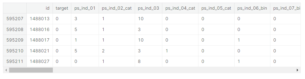
We indeed see the following
- binary variables
- categorical variables of which the category values are integers
- other variables with integer or float values
- variables with -1 representing missing values
- the target variable and an ID variable
Let's look at the number of rows and columns in the train data.
train.shape
(595212, 59)We have 59 variables and 595.212 rows. Let's see if we have the same number of variables in the test data.
Let's see if there are duplicate rows in the training data.
- 테스트 세트에서 서로 같은 수의 변수가 있는지 확인
- 훈련 세트에서 중복된 행 있는지 확인
train.drop_duplicates()
train.shape
(595212, 59)No duplicate rows, so that's fine.
- drop_duplicates()는 내용이 중복되는 행을 제거, subset에 입력된 행을 기준으로 중복값을 제거하며 아무것도 입력하지 않고 ()만 할 경우 모든 열에 대해 값이 중복인 행을 제거
- 현재 훈련 세트에서는 drop_duplicate 데이터를 적용해도 데이터 행과 열의 수가 동일하게 나옴 >> 중복값이 없음
test.shape(892816, 58)We are missing one variable in the test set, but this is the target variable. So that's fine.
Let's now invesigate how many variables of each type we have.
- 테스트 세트에서 한 변수가 누락되어있지만, 이는 표적 변수(target variable)이므로 신경쓰지 않아도 괜찮음
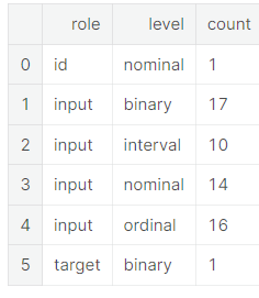
So later on we can create dummy variables for the 14 categorical variables. The bin variables are already binary and do not need dummification.
- dummy variable is one that takes the values 0 or 1 to indicate the absence or presence of some categorical effect that may be expected to shift the outcome. (출처 : https://en.wikipedia.org/wiki/Dummy_variable_(statistics))
- dummy varable이란 모델링에 영향을 주고 결과를 바꿀 수 있는 있는 범주형 데이터의 존재 또는 부재를 나타내기 위해 0과 1로 나누어준 것
train.info()
<class 'pandas.core.frame.DataFrame'>
RangeIndex: 595212 entries, 0 to 595211
Data columns (total 59 columns):
id                595212 non-null int64
target            595212 non-null int64
ps_ind_01         595212 non-null int64
ps_ind_02_cat     595212 non-null int64
ps_ind_03         595212 non-null int64
ps_ind_04_cat     595212 non-null int64
ps_ind_05_cat     595212 non-null int64
ps_ind_06_bin     595212 non-null int64
ps_ind_07_bin     595212 non-null int64
ps_ind_08_bin     595212 non-null int64
ps_ind_09_bin     595212 non-null int64
ps_ind_10_bin     595212 non-null int64
ps_ind_11_bin     595212 non-null int64
ps_ind_12_bin     595212 non-null int64
ps_ind_13_bin     595212 non-null int64
ps_ind_14         595212 non-null int64
ps_ind_15         595212 non-null int64
ps_ind_16_bin     595212 non-null int64
ps_ind_17_bin     595212 non-null int64
ps_ind_18_bin     595212 non-null int64
ps_reg_01         595212 non-null float64
ps_reg_02         595212 non-null float64
ps_reg_03         595212 non-null float64
ps_car_01_cat     595212 non-null int64
ps_car_02_cat     595212 non-null int64
ps_car_03_cat     595212 non-null int64
ps_car_04_cat     595212 non-null int64
ps_car_05_cat     595212 non-null int64
ps_car_06_cat     595212 non-null int64
ps_car_07_cat     595212 non-null int64
ps_car_08_cat     595212 non-null int64
ps_car_09_cat     595212 non-null int64
ps_car_10_cat     595212 non-null int64
ps_car_11_cat     595212 non-null int64
ps_car_11         595212 non-null int64
ps_car_12         595212 non-null float64
ps_car_13         595212 non-null float64
ps_car_14         595212 non-null float64
ps_car_15         595212 non-null float64
ps_calc_01        595212 non-null float64
ps_calc_02        595212 non-null float64
ps_calc_03        595212 non-null float64
ps_calc_04        595212 non-null int64
ps_calc_05        595212 non-null int64
ps_calc_06        595212 non-null int64
ps_calc_07        595212 non-null int64
ps_calc_08        595212 non-null int64
ps_calc_09        595212 non-null int64
ps_calc_10        595212 non-null int64
ps_calc_11        595212 non-null int64
ps_calc_12        595212 non-null int64
ps_calc_13        595212 non-null int64
ps_calc_14        595212 non-null int64
ps_calc_15_bin    595212 non-null int64
ps_calc_16_bin    595212 non-null int64
ps_calc_17_bin    595212 non-null int64
ps_calc_18_bin    595212 non-null int64
ps_calc_19_bin    595212 non-null int64
ps_calc_20_bin    595212 non-null int64
dtypes: float64(10), int64(49)
memory usage: 267.9 MB
Again, with the info() method we see that the data type is integer or float. No null values are present in the data set. That's normal because missing values are replaced by -1. We'll look into that later.
- info() 메소드를 통해 데이터 타입이 integer인지 float인지 확인 가능
- 누락된 값들 (null 데이터들)을 -1로 대체했기 때문에 현재 데이터세세 null 데이터가 없는 것으로 보임
Metadata
To facilitate the data management, we'll store meta-information about the variables in a DataFrame. This will be helpful when we want to select specific variables for analysis, visualization, modeling, ...
Concretely we will store:
- role: input, ID, target
- level: nominal, interval, ordinal, binary
- keep: True or False
- dtype: int, float, str
- 데이터 관리를 용이하게 하기 위해, 변수들에 대한 meta-information을 데이터프레임에 저장할 것 >> 분석, 시각화, 모델링 등을 위해 특정한 변수 지정할 때 편리
data = []
for f in train.columns:
    # Defining the role
    if f == 'target':
        role = 'target'
    elif f == 'id':
        role = 'id'
    else:
        role = 'input'

    # Defining the level
    if 'bin' in f or f == 'target':
        level = 'binary'
    elif 'cat' in f or f == 'id':
        level = 'nominal'
    elif train[f].dtype == float:
        level = 'interval'
    elif train[f].dtype == int:
        level = 'ordinal'

        # Initialize keep to True for all variables except for id
    keep = True
    if f == 'id':
        keep = False

    # Defining the data type
    dtype = train[f].dtype

    # Creating a Dict that contains all the metadata for the variable
    f_dict = {
        'varname': f,
        'role': role,
        'level': level,
        'keep': keep,
        'dtype': dtype
    }
    data.append(f_dict)

meta = pd.DataFrame(data, columns=['varname', 'role', 'level', 'keep', 'dtype'])
meta.set_index('varname', inplace=True)- 모든 데이터들마다 role(input/ID/target), level(nominal/interval/ordinal/binary), keep(True/False), dtype(int, float, str) 정해줌
- >> meta 데이터프레임에 넣어줌
- nominal : 순서를 매길 수 없고 그냥 셀 수만 있는 명목형 데이터 / interval : 서로 같은 간격으로 떨어져있는 데이터들을 의미, 시간 개념으로 많이 쓰임, 항상 수치형 데이터 / binary : 0과 1로만 이루어진 데이터 / ordinal : 순서가 정해진 범주형 데이터
meta

- 모든 데이터들을 가지고 role, level, keep, dtype을 구분해줌
- 일반적으로 데이터셋의 메타정보라고 하면 데이터 셋의 각 칼럼에 대한 정보로서 각 칼럼의 용도가 무엇이며, 데이터 종류는 무엇이며(연속형, 범주형 등), 데이터 타입은 무엇이며(정수, 문자, 소수 등)에 대한 정보를 의미 >> 메티 정보를 따로 관리하기 위한 데이터 프레임을 만들면 분석하는데 도움이 됨
Example to extract all nominal variables that are not dropped.
- 드랍되지 않은 모든 nominal 변수들 추출
meta[(meta.level == 'nominal') & (meta.keep)].index- meta에서 level이 nominal이고 keep이 true인 인덱스 출력
Index(['ps_ind_02_cat', 'ps_ind_04_cat', 'ps_ind_05_cat', 'ps_car_01_cat',
       'ps_car_02_cat', 'ps_car_03_cat', 'ps_car_04_cat', 'ps_car_05_cat',
       'ps_car_06_cat', 'ps_car_07_cat', 'ps_car_08_cat', 'ps_car_09_cat',
       'ps_car_10_cat', 'ps_car_11_cat'],
      dtype='object', name='varname')
Below the number of variables per role and level are displayed.
pd.DataFrame({'count' : meta.groupby(['role', 'level'])['role'].size()}).reset_index()
- meta.groupby(['role', 'level'])['role'].size() >> groupby에 사용된 칼럼을 밖에서 사용하여 size()로 실행, 해당 그룹의 row가 몇개인지 보기 위함. meta.groupby(['role','level']).count()라고 해도 칼럼만 다를 뿐 출력되는 숫자는 일치
- 단지 count()를 사용하면 결과에서 카운트 값을 할당할 칼럼명이 나머지 칼럼들에 다 할당되는것이고, size()로 실행하면 카운트 값을 할당할 칼럼은 없이 그냥 카운트된 수치만 반환.
- count()는 칼럼의 NaN값을 카운트하지 않는 반면, size()는 칼럼의 NaN값까지 포함하여 카운트
- pd.DataFrame으로 데이터프레임 만들기, 'count'라는 인덱스 지정
- groupby().size() >> 각 그룹의 사이즈 출력
- 밑의 groupby 표에서 한 role에 속하는 각 level 안에 몇 개의 데이터가 들어있는지 나타내줌
- reset_index() >> 인덱스 행 새로 추가
Descriptive statistics
- 기술 통계량
We can also apply the describe method on the dataframe. However, it doesn't make much sense to calculate the mean, std, ... on categorical variables and the id variable. We'll explore the categorical variables visually later.
Thanks to our meta file we can easily select the variables on which we want to compute the descriptive statistics. To keep things clear, we'll do this per data type.
- 범주형 데이터는 추후에 시각화 시킬 것
Interval variables
v = meta[(meta.level == 'interval') & (meta.keep)].index
train[v].describe()- meta에서 level이 interval이고 keep가 True인 feature들에(feature들이 인덱스) v라는 이름의 인덱스 부여
- Dataframe.index로 데이터프레임의 인덱스를 조작
- train의 v 인덱스의 요약통계치

reg variables
- only ps_reg_03 has missing values
- the range (min to max) differs between the variables. We could apply scaling (e.g. StandardScaler), but it depends on the classifier we will want to use.
- ps_reg_03에만 -1 존재, 즉 누락된 값이 있음
- 최댓값과 최솟값의 범위가 변수들 사이에서 다르게 나타남 >> 데이터 스케일링을 진행할 수 있지만 우리가 사용하기를 원하는 구분기에 의해 스케일링 여부가 결정됨
car variables
- ps_car_12 and ps_car_15 have missing values
- again, the range differs and we could apply scaling.
calc variables
- no missing values
- this seems to be some kind of ratio as the maximum is 0.9
- all three _calc variables have very similar distributions
- 세 calc 변수들의 최대치가 모두 0.9이기 때문에 일종의 비율 같은 것이라고 볼 수 있음, 세 calc 변수들은 굉장히 유사한 분포를 나타내고 있음 (사분위수를 통해 알 수 있음!)
Overall, we can see that the range of the interval variables is rather small. Perhaps some transformation (e.g. log) is already applied in order to anonymize the data?
- 전반적으로, interval 변수들의 범위가 다소 작다는 사실을 알 수 있음 >> 아마 log와 같은 조치가 데이터 익명화를 위해 취해졌을 것으로 보임 (데이터 익명화 : 데이터셋에서 식별 가능한 데이터를 제거하거나 암호화하여 삭제하는 방법)
Ordinal variables
v = meta[(meta.level == 'ordinal') & (meta.keep)].index
train[v].describe()- meta 데이터셋에서 level이 ordinal이면서 keep이 True인 feature들의 인덱스에 v라는 이름 부여
- train[v]의 요약통계치 제공
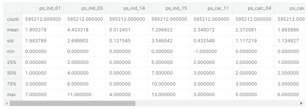
- Only one missing variable: ps_car_11
- We could apply scaling to deal with the different ranges
Binary variables
v = meta[(meta.level == 'binary') & (meta.keep)].index
train[v].describe()- meta 데이터셋에서 level이 binary이면서 keep이 True인 feature들의 인덱스에 v라는 이름 부여
- train[v]의 요약통계치 제공
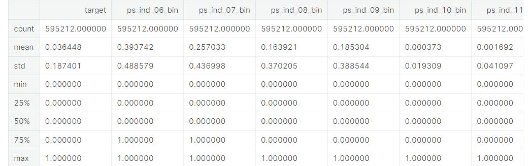
- Apriori in the train data is 3.645%, which is strongly imbalanced.
- From the means we can conclude that for most variables the value is zero in most cases.
- Apriori 알고리즘 >> 훈련세트에서 target칼럼의 값은 0 또는 1인데, 이 데이터의 경우 1값을 갖는 경우보다 0값을 갖는 경우가 훨씬 빈번함. 따라서 target이라는 칼럼은 데이터가 imbalance하다는 것(0이 너무 많음), 칼럼값이 골고루 분포하지 않고 특정 값에 많이 치우쳐져있음
- 위 데이터는 굉장히 불균등하게 분포하고 있으며, 범위를 보면 대부분의 변수들의 값이 0임을 알 수 있음
Handling imbalanced classes
- 불균등한 classes 조정하기
As we mentioned above the proportion of records with target=1 is far less than target=0. This can lead to a model that has great accuracy but does have any added value in practice. Two possible strategies to deal with this problem are:
- oversampling records with target=1
- undersampling records with target=0
There are many more strategies of course and MachineLearningMastery.com gives a nice overview. As we have a rather large training set, we can go for undersampling.
- target 값이 1인 데이터들보다 0인 데이터가 현저히 많기 때문에, 이를 모델에게 학습시키면 높은 정확도를 갖지만 훈련 시에 부가 가치 값을 얻게 된다...??
- 해결 방법 >> target=1인 기록들을 oversempling하거나 target=0인 기록들을 undersempling(여기서는 후자 사용)
- 오버샘플링(Oversampling)은 필요한 샘플링 개수보다 더 많은 샘플링을 수행하고 평균을 하는 기법이다. 예를 들면, 1초에 100개의 샘플링이 필요할 때 1초에 400개를 샘플링하고 4개 샘플마다 4개 샘플을 평균하여 100개 샘플을 계산한다. 오버 샘플링은 낮은 비율 클래스의 데이터 수를 늘림으로써 데이터 불균형을 해소하는 아이디어 (from https://article2.tistory.com/780)
- 언더 샘플링은 불균형한 데이터 셋에서 높은 비율을 차지하던 클래스의 데이터 수를 줄임으로써 데이터 불균형을 해소하는 아이디어 (from https://hwi-doc.tistory.com/entry/%EC%96%B8%EB%8D%94-%EC%83%98%ED%94%8C%EB%A7%81Undersampling%EA%B3%BC-%EC%98%A4%EB%B2%84-%EC%83%98%ED%94%8C%EB%A7%81Oversampling)
- 현재 데이터셋 타겟에 0이 1보다 훨씬 많음 예를 들어 칼럼값 100개중 97개가 0이면 나머지 칼럼으로 모델을 학습시키지 않고 그냥 항상 target이 0이라고 예측해도 그 정확도가 97퍼센트가 될 정도로 높음. 이런 경우에는 모델은 학습이 제대로 되어있지 않지만 학습 데이터의 불균형 때문에 예측도가 높게 나타남 >> 이러한 경우를 피하기 위해 데이터의 균형을 맞춰줘야 함.
desired_apriori=0.10

# Get the indices per target value
idx_0 = train[train.target == 0].index
idx_1 = train[train.target == 1].index

# Get original number of records per target value
nb_0 = len(train.loc[idx_0])
nb_1 = len(train.loc[idx_1])

# Calculate the undersampling rate and resulting number of records with target=0
undersampling_rate = ((1-desired_apriori)*nb_1)/(nb_0*desired_apriori)
undersampled_nb_0 = int(undersampling_rate*nb_0)
print('Rate to undersample records with target=0: {}'.format(undersampling_rate))
print('Number of records with target=0 after undersampling: {}'.format(undersampled_nb_0))

# Randomly select records with target=0 to get at the desired a priori
undersampled_idx = shuffle(idx_0, random_state=37, n_samples=undersampled_nb_0)

# Construct list with remaining indices
idx_list = list(undersampled_idx) + list(idx_1)

# Return undersample data frame
train = train.loc[idx_list].reset_index(drop=True)- idx_0은 target값이 0인 데이터들의 인덱스, idx_1은 target값이 1인 데이터들의 인덱스
- nb_0은 idx_0의 길이(target값이 0인 데이터들의 개수), nb_1은 idx_1의 길이(target값이 0인 데이터들의 개수)
- Apriori는 빈발항목집합을 추출하는 것이 원리입니다. 여기서 빈발항목집합이란? 최소지지도 이상을 갖는 항목집합을 의미합니다. 모든 항목집합의 대한 복잡한 계산량을 줄이기 위해 최소 지지도를 정해서 그 이상의 값만 찾은 후 연관규칙을 생성하게 됩니다. (from https://jaaamj.tistory.com/114)
- undersampling_rate = (1-0.10)*nb_1 / nb_0*0.10, undersampled_nb_0 >> undersampling_rate*nb_0을 정수형으로 변환한 것
- 문자열을 정의하고 나서 .format() 매소드를 사용해서 인수로 {} 개수 만큼 문자열이나, 숫자를 추가 해주면 해당 값이 차례대로 문자열에 들어간다. (from https://m.blog.naver.com/sw4r/221975908756)
- random_state 매개변수 : 자체적으로 랜덤 시드 지정
- undersampled_idx(undersampled된 target=0 데이터), idx_list(undersampled_idx와 idx_1을 합친 것)
- reset_index 메서드를 호출할 때 인수 drop=True 로 설정하면 인덱스 열을 보통의 자료열로 올리는 것이 아니라 그냥 버리게 된다.
- train데이터프레임에 idx_list(undersampled_idx와 idx_1을 합친 것)에 속하는 데이터들만 넣음
Rate to undersample records with target=0: 0.34043569687437886
Number of records with target=0 after undersampling: 195246
Data Quality Checks
Checking missing values
Missings are represented as -1
- 결측치 확인 >> -1로 대체되어있음
vars_with_missing = []

for f in train.columns:
    missings = train[train[f] == -1][f].count()
    if missings > 0:
        vars_with_missing.append(f)
        missings_perc = missings/train.shape[0]

        print('Variable {} has {} records ({:.2%}) with missing values'.format(f, missings, missings_perc))

print('In total, there are {} variables with missing values'.format(len(vars_with_missing)))- vars_with_missing = [] 리스트 생성
- for문 생성, f는 train의 column들. -1이 있으면 missings변수 ++1
- missings변수 >0 (즉 한 칼럼에 -1이 하나라도 있으면) >> vars_with_missing 리스트에 -1인 train column 추가, 전체 트레인에 비해 각 칼럼에 결측치가 얼마나 있는지 그 비율을 missings_perc로 나타냄
Variable ps_ind_02_cat has 103 records (0.05%) with missing values
Variable ps_ind_04_cat has 51 records (0.02%) with missing values
Variable ps_ind_05_cat has 2256 records (1.04%) with missing values
Variable ps_reg_03 has 38580 records (17.78%) with missing values
Variable ps_car_01_cat has 62 records (0.03%) with missing values
Variable ps_car_02_cat has 2 records (0.00%) with missing values
Variable ps_car_03_cat has 148367 records (68.39%) with missing values
Variable ps_car_05_cat has 96026 records (44.26%) with missing values
Variable ps_car_07_cat has 4431 records (2.04%) with missing values
Variable ps_car_09_cat has 230 records (0.11%) with missing values
Variable ps_car_11 has 1 records (0.00%) with missing values
Variable ps_car_14 has 15726 records (7.25%) with missing values
In total, there are 12 variables with missing values- ps_car_03_cat and ps_car_05_cat have a large proportion of records with missing values. Remove these variables.
- For the other categorical variables with missing values, we can leave the missing value -1 as such.
- ps_reg_03 (continuous) has missing values for 18% of all records. Replace by the mean.
- ps_car_11 (ordinal) has only 5 records with misisng values. Replace by the mode.
- ps_car_12 (continuous) has only 1 records with missing value. Replace by the mean.
- ps_car_14 (continuous) has missing values for 7% of all records. Replace by the mean.
# Dropping the variables with too many missing values
vars_to_drop = ['ps_car_03_cat', 'ps_car_05_cat']
train.drop(vars_to_drop, inplace=True, axis=1)
meta.loc[(vars_to_drop),'keep'] = False  # Updating the meta

# Imputing with the mean or mode
mean_imp = Imputer(missing_values=-1, strategy='mean', axis=0)
mode_imp = Imputer(missing_values=-1, strategy='most_frequent', axis=0)
train['ps_reg_03'] = mean_imp.fit_transform(train[['ps_reg_03']]).ravel()
train['ps_car_12'] = mean_imp.fit_transform(train[['ps_car_12']]).ravel()
train['ps_car_14'] = mean_imp.fit_transform(train[['ps_car_14']]).ravel()
train['ps_car_11'] = mode_imp.fit_transform(train[['ps_car_11']]).ravel()- 결측치가 너무 많은 칼럼은 훈련 세트에서 삭제 (원본 데이터에 반영, index를 drop하려면 axis=0으로 설정하고, 컬럼을 drop하려면 axis=1로 설정)
- axis=0은 행, axis=1은 열 방향으로 동작 (출처 https://hogni.tistory.com/49)
- meta 데이터셋에서, 훈련 세트에서 지운 feature들의 keep을 False로 바꿔줌(업데이트)
- mean_imp는 결측치를 평균(mean)으로 대체한 것, mode_imp는 결측치를 최빈값(most_frequent)으로 대체한 것
- Imputer(missing_values, strategy, axis, verbose, copy) : 결측치를 대체시켜주는 사이킷런 전처리 함수
- missing_values : default = 'NaN', 해당 데이터 내에서 결측치 값, 예를 들어, 만약 NaN 대신, 결측치가 -1로 채워져 있다면, missing_values = -1 로 작성해야 한다.
- strategy : 결측치를 대체할 값, default = 'mean', median, most_frequent 등도 사용 가능하다.
- axis : 방향 설정, axis = 0 or 1
- fit()은 데이터를 학습시키는 메서드이고 transform()은 실제로 학습시킨 것을 적용하는 메서드, fit_transform()은 말그대로 fit()과 transform()을 한번에 처리할 수 있게 하는 메서드인데 조심해야 하는 것은 테스트 데이터에는 fit_transform() 메서드를 쓰면 안된다는 것 (출처 : https://for-my-wealthy-life.tistory.com/18)
- 결측치가 있는 feature들에 대해, 결측치를 평균 또는 최빈값으로 대체시킴
Checking the cardinality of the categorical variables
- cardinality : 전체 행에 대한 특정 컬럼의 중복 수치를 나타내는 지표 (출처 : https://itholic.github.io/database-cardinality/)
Cardinality refers to the number of different values in a variable. As we will create dummy variables from the categorical variables later on, we need to check whether there are variables with many distinct values. We should handle these variables differently as they would result in many dummy variables.
- 범주형 변수는 추후에 dummy 변수로 만들어줄 것이기 때문에, 범주형 데이터 안에 서로 다른 값들이 얼마나 있는지 확인해야 할 필요가 있음
v = meta[(meta.level == 'nominal') & (meta.keep)].index

for f in v:
    dist_values = train[f].value_counts().shape[0]
print('Variable {} has {} distinct values'.format(f, dist_values))- level이 nominal이면서 keep가 True인 feature들의 인덱스에 v라는 이름 부여
Variable ps_ind_02_cat has 5 distinct values
Variable ps_ind_04_cat has 3 distinct values
Variable ps_ind_05_cat has 8 distinct values
Variable ps_car_01_cat has 13 distinct values
Variable ps_car_02_cat has 3 distinct values
Variable ps_car_04_cat has 10 distinct values
Variable ps_car_06_cat has 18 distinct values
Variable ps_car_07_cat has 3 distinct values
Variable ps_car_08_cat has 2 distinct values
Variable ps_car_09_cat has 6 distinct values
Variable ps_car_10_cat has 3 distinct values
Variable ps_car_11_cat has 104 distinct values- 각 범주형 데이터 feature들에 서로 다른 변수가 몇 개 존재하는지 출력
Only ps_car_11_cat has many distinct values, although it is still reasonable.
EDIT: nickycan made an excellent remark on the fact that my first solution could lead to data leakage. He also pointed me to another kernel made by oliver which deals with that. I therefore replaced this part with the kernel of oliver. All credits go to him. It is so great what you can learn by participating in the Kaggle competitions :)
# Script by https://www.kaggle.com/ogrellier
# Code: https://www.kaggle.com/ogrellier/python-target-encoding-for-categorical-features
def add_noise(series, noise_level):
    return series * (1 + noise_level * np.random.randn(len(series)))

def target_encode(trn_series=None,
                  tst_series=None,
                  target=None,
                  min_samples_leaf=1,
                  smoothing=1,
                  noise_level=0):
    """
    Smoothing is computed like in the following paper by Daniele Micci-Barreca
    https://kaggle2.blob.core.windows.net/forum-message-attachments/225952/7441/high%20cardinality%20categoricals.pdf
    trn_series : training categorical feature as a pd.Series
    tst_series : test categorical feature as a pd.Series
    target : target data as a pd.Series
    min_samples_leaf (int) : minimum samples to take category average into account
    smoothing (int) : smoothing effect to balance categorical average vs prior
    """
    assert len(trn_series) == len(target)
    assert trn_series.name == tst_series.name
    temp = pd.concat([trn_series, target], axis=1)
    # Compute target mean
    averages = temp.groupby(by=trn_series.name)[target.name].agg(["mean", "count"])
    # Compute smoothing
    smoothing = 1 / (1 + np.exp(-(averages["count"] - min_samples_leaf) / smoothing))
    # Apply average function to all target data
    prior = target.mean()
    # The bigger the count the less full_avg is taken into account
    averages[target.name] = prior * (1 - smoothing) + averages["mean"] * smoothing
    averages.drop(["mean", "count"], axis=1, inplace=True)
    # Apply averages to trn and tst series
    ft_trn_series = pd.merge(
        trn_series.to_frame(trn_series.name),
        averages.reset_index().rename(columns={'index': target.name, target.name: 'average'}),
        on=trn_series.name,
        how='left')['average'].rename(trn_series.name + '_mean').fillna(prior)
    # pd.merge does not keep the index so restore it
    ft_trn_series.index = trn_series.index
    ft_tst_series = pd.merge(
        tst_series.to_frame(tst_series.name),
        averages.reset_index().rename(columns={'index': target.name, target.name: 'average'}),
        on=tst_series.name,
        how='left')['average'].rename(trn_series.name + '_mean').fillna(prior)
    # pd.merge does not keep the index so restore it
    ft_tst_series.index = tst_series.index
    return add_noise(ft_trn_series, noise_level), add_noise(ft_tst_series, noise_level)
train_encoded, test_encoded = target_encode(train["ps_car_11_cat"],
test["ps_car_11_cat"],
target=train.target,
min_samples_leaf=100,
smoothing=10,
noise_level=0.01)
train['ps_car_11_cat_te'] = train_encoded
train.drop('ps_car_11_cat', axis=1, inplace=True)
meta.loc['ps_car_11_cat','keep'] = False # Updating the meta
test['ps_car_11_cat_te'] = test_encoded
test.drop('ps_car_11_cat', axis=1, inplace=True)
Exploratory Data Visualization
Categorical variables
Let's look into the categorical variables and the proportion of customers with target = 1
- 범주형 데이터에서 target=1인 데이터들의 비율
v = meta[(meta.level == 'nominal') & (meta.keep)].index

for f in v:
    plt.figure()
    fig, ax = plt.subplots(figsize=(20,10))
    # Calculate the percentage of target=1 per category value
    cat_perc = train[[f, 'target']].groupby([f],as_index=False).mean()
    cat_perc.sort_values(by='target', ascending=False, inplace=True)
    # Bar plot
    # Order the bars descending on target mean
    sns.barplot(ax=ax, x=f, y='target', data=cat_perc, order=cat_perc[f])
    plt.ylabel('% target', fontsize=18)
    plt.xlabel(f, fontsize=18)
    plt.tick_params(axis='both', which='major', labelsize=18)
plt.show();- 범주형 데이터들의 feature별 target값 평균으로 groupby하고 이를 sort_values로 정렬

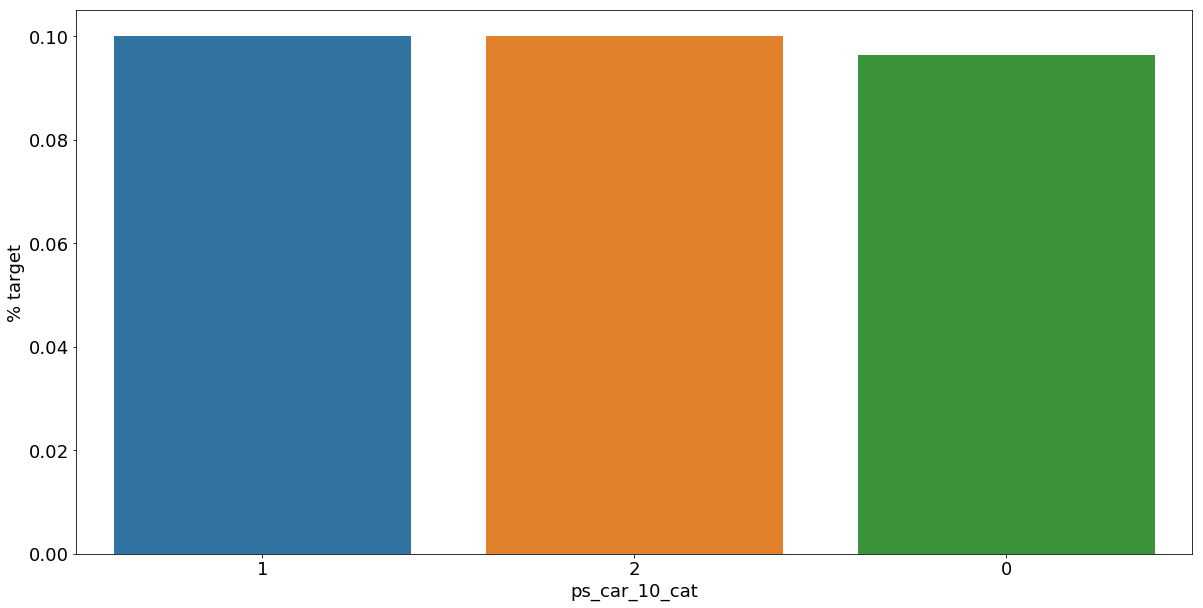


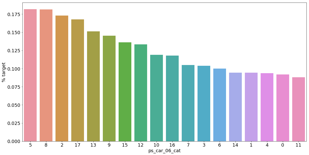

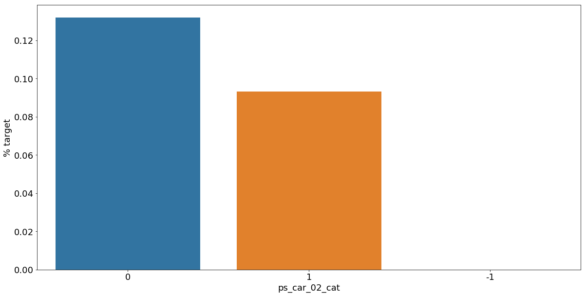

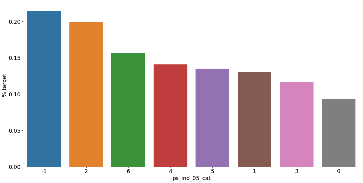

As we can see from the variables with missing values, it is a good idea to keep the missing values as a separate category value, instead of replacing them by the mode for instance. The customers with a missing value appear to have a much higher (in some cases much lower) probability to ask for an insurance claim.
- 결측값들은 다른 것으로 대체하기보다 특정한 범주형 데이터로서 따로 분리하는 것이 좋은 아이디어이다.
Interval variables
Checking the correlations between interval variables. A heatmap is a good way to visualize the correlation between variables. The code below is based on an example by Michael Waskom
Plotting a diagonal correlation matrix — seaborn 0.12.2 documentation
Plotting a diagonal correlation matrix seaborn components used: set_theme(), diverging_palette(), heatmap() from string import ascii_letters import numpy as np import pandas as pd import seaborn as sns import matplotlib.pyplot as plt sns.set_theme(style="w
seaborn.pydata.org
- interval variables는 각 변수간의 상관관계를 heatmap으로 표현할 것
def corr_heatmap(v):
    correlations = train[v].corr()

    # Create color map ranging between two colors
    cmap = sns.diverging_palette(220, 10, as_cmap=True)

    fig, ax = plt.subplots(figsize=(10,10))
    sns.heatmap(correlations, cmap=cmap, vmax=1.0, center=0, fmt='.2f',
                square=True, linewidths=.5, annot=True, cbar_kws={"shrink": .75})
    plt.show();

v = meta[(meta.level == 'interval') & (meta.keep)].index
corr_heatmap(v)
There are a strong correlations between the variables:
- ps_reg_02 and ps_reg_03 (0.7)
- ps_car_12 and ps_car13 (0.67)
- ps_car_12 and ps_car14 (0.58)
- ps_car_13 and ps_car15 (0.67)
Seaborn has some handy plots to visualize the (linear) relationship between variables. We could use a pairplot to visualize the relationship between the variables. But because the heatmap already showed the limited number of correlated variables, we'll look at each of the highly correlated variables separately.
NOTE: I take a sample of the train data to speed up the process.
- Seaborn의 pairplot을 이용하여 특별히 높은 상관성을 가지고 있는 변수들을 시각화
s = train.sample(frac=0.1)
- frac 매개변수로 무작위 표본 추출
ps_reg_02 and ps_reg_03
As the regression line shows, there is a linear relationship between these variables. Thanks to the hue parameter we can see that the regression lines for target=0 and target=1 are the same.
sns.lmplot(x='ps_reg_02', y='ps_reg_03', data=s, hue='target', palette='Set1', scatter_kws={'alpha':0.3})
plt.show()
- 두 변수에서 target이 0일때와 1일때의 선형 회귀 함수는 동일한 것으로 나타남(target 결과가 같다)
ps_car_12 and ps_car_13
sns.lmplot(x='ps_car_12', y='ps_car_13', data=s, hue='target', palette='Set1', scatter_kws={'alpha':0.3})
plt.show()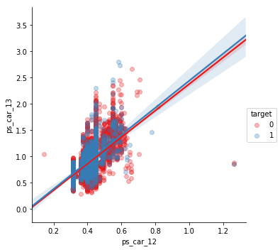
ps_car_12 and ps_car_14
sns.lmplot(x='ps_car_12', y='ps_car_14', data=s, hue='target', palette='Set1', scatter_kws={'alpha':0.3})
plt.show()
ps_car_13 and ps_car_15
sns.lmplot(x='ps_car_15', y='ps_car_13', data=s, hue='target', palette='Set1', scatter_kws={'alpha':0.3})
plt.show()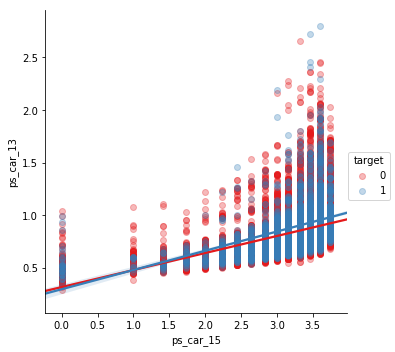
Allright, so now what? How can we decide which of the correlated variables to keep? We could perform Principal Component Analysis (PCA) on the variables to reduce the dimensions. In the AllState Claims Severity Competition I made this kernel to do that. But as the number of correlated variables is rather low, we will let the model do the heavy-lifting.
Reducing number of numerical features with PCA
Explore and run machine learning code with Kaggle Notebooks | Using data from Allstate Claims Severity
www.kaggle.com
Checking the correlations between ordinal variables
v = meta[(meta.level == 'ordinal') & (meta.keep)].index
corr_heatmap(v)
- 순서가 있는 범주형 데이터들 사이의 상관관계를 나타냄
For the ordinal variables we do not see many correlations. We could, on the other hand, look at how the distributions are when grouping by the target value.
Feature engineering
Creating dummy variables
The values of the categorical variables do not represent any order or magnitude. For instance, category 2 is not twice the value of category 1. Therefore we can create dummy variables to deal with that. We drop the first dummy variable as this information can be derived from the other dummy variables generated for the categories of the original variable.
v = meta[(meta.level == 'nominal') & (meta.keep)].index
print('Before dummification we have {} variables in train'.format(train.shape[1]))
train = pd.get_dummies(train, columns=v, drop_first=True)
print('After dummification we have {} variables in train'.format(train.shape[1]))
Before dummification we have 57 variables in train
After dummification we have 109 variables in trainSo, creating dummy variables adds 52 variables to the training set.
- 범주형 데이터들을 dummy variables로 만들어줌
Creating interaction variables
v = meta[(meta.level == 'interval') & (meta.keep)].index
poly = PolynomialFeatures(degree=2, interaction_only=False, include_bias=False)
interactions = pd.DataFrame(data=poly.fit_transform(train[v]), columns=poly.get_feature_names(v))
interactions.drop(v, axis=1, inplace=True)  # Remove the original columns
# Concat the interaction variables to the train data
print('Before creating interactions we have {} variables in train'.format(train.shape[1]))
train = pd.concat([train, interactions], axis=1)
print('After creating interactions we have {} variables in train'.format(train.shape[1]))
Before creating interactions we have 109 variables in train
After creating interactions we have 164 variables in trainThis adds extra interaction variables to the train data. Thanks to the get_feature_names method we can assign column names to these new variables.
- PolynomialFeatures >> 다항회귀 (데이터의 분포가 곡선으로 나타나 선형회귀로 해결하기 어려울 때 사용)
- degree 옵션으로 각 특성의 차수를 조절, include_bias 옵션은 True로 할 경우 0차항(1)도 함께 만든다. (출처 : https://inuplace.tistory.com/515)
- 다항차수는 적용하지 않고, 오직 교호작용 효과만을 분석하려면 interaction_only=True 옵션을 설정해주면 됩니다. degree를 가지고 교호작용을 몇 개 수준까지 볼 지 설정해줄 수 있습니다 (출처 : https://rfriend.tistory.com/274)
- 교호작용 효과란 두 개 이상의 요인의 조합에서 생기는 효과를 의미하는데 한 요인이 결과에 미치는 영향이 다른 요인의 상태에 따라 달라지는 상황에서 나타난다. (출처 : https://jkwra.or.kr/articles/pdf/rjVq/kwra-2018-051-11S-3.pdf)
Feature selection
Removing features with low or zero variance
Personally, I prefer to let the classifier algorithm chose which features to keep. But there is one thing that we can do ourselves. That is removing features with no or a very low variance. Sklearn has a handy method to do that: VarianceThreshold. By default it removes features with zero variance. This will not be applicable for this competition as we saw there are no zero-variance variables in the previous steps. But if we would remove features with less than 1% variance, we would remove 31 variables.
- variace가 1퍼센트 미만인 feature 제거
selector = VarianceThreshold(threshold=.01)
selector.fit(train.drop(['id', 'target'], axis=1)) # Fit to train without id and target variables

f = np.vectorize(lambda x : not x) # Function to toggle boolean array elements

v = train.drop(['id', 'target'], axis=1).columns[f(selector.get_support())]
print('{} variables have too low variance.'.format(len(v)))
print('These variables are {}'.format(list(v)))
28 variables have too low variance.
These variables are ['ps_ind_10_bin', 'ps_ind_11_bin', 'ps_ind_12_bin', 'ps_ind_13_bin', 'ps_car_12', 'ps_car_14', 'ps_car_11_cat_te', 'ps_ind_05_cat_2', 'ps_ind_05_cat_5', 'ps_car_01_cat_1', 'ps_car_01_cat_2', 'ps_car_04_cat_3', 'ps_car_04_cat_4', 'ps_car_04_cat_5', 'ps_car_04_cat_6', 'ps_car_04_cat_7', 'ps_car_06_cat_2', 'ps_car_06_cat_5', 'ps_car_06_cat_8', 'ps_car_06_cat_12', 'ps_car_06_cat_16', 'ps_car_06_cat_17', 'ps_car_09_cat_4', 'ps_car_10_cat_1', 'ps_car_10_cat_2', 'ps_car_12^2', 'ps_car_12 ps_car_14', 'ps_car_14^2']- Variance threshold는 말 그대로 변수의 분산이 지정한 threshold 보다 작으면 제거하는 방법이다. 변수의 분산이 너무 작으면 타겟을 예측하는 성능이 낮아진다고 판단하는데, 어떤 변수의 분산이 작으면 변수의 각 값들이 타겟에 미치는 영향의 차이는 미비하기 때문이다. 이러한 이유로 feature을 선택할 때 이 방법을 사용하기도 한다. (출처 : https://hyewonleess.github.io/ml/feature_selection/)
We would lose rather many variables if we would select based on variance. But because we do not have so many variables, we'll let the classifier chose. For data sets with many more variables this could reduce the processing time.
Sklearn also comes with other feature selection methods. One of these methods is SelectFromModel in which you let another classifier select the best features and continue with these. Below I'll show you how to do that with a Random Forest.
Selecting features with a Random Forest and SelectFromModel
Here we'll base feature selection on the feature importances of a random forest. With Sklearn's SelectFromModel you can then specify how many variables you want to keep. You can set a threshold on the level of feature importance manually. But we'll simply select the top 50% best variables.
The code in the cell below is borrowed from the GitHub repo of Sebastian Raschka. This repo contains code samples of his book Python Machine Learning, which is an absolute must to read.
X_train = train.drop(['id', 'target'], axis=1)
y_train = train['target']

feat_labels = X_train.columns

rf = RandomForestClassifier(n_estimators=1000, random_state=0, n_jobs=-1)

rf.fit(X_train, y_train)
importances = rf.feature_importances_

indices = np.argsort(rf.feature_importances_)[::-1]

for f in range(X_train.shape[1]):
    print("%2d) %-*s %f" % (f + 1, 30,feat_labels[indices[f]], importances[indices[f]]))
1) ps_car_11_cat_te 0.021243
2) ps_car_13 0.017344
3) ps_car_12 ps_car_13 0.017267
4) ps_car_13^2 0.017221
5) ps_car_13 ps_car_14 0.017166
6) ps_reg_03 ps_car_13 0.017075
7) ps_car_13 ps_car_15 0.016905
8) ps_reg_01 ps_car_13 0.016783
9) ps_reg_03 ps_car_14 0.016195
10) ps_reg_03 ps_car_12 0.015519
11) ps_reg_03 ps_car_15 0.015187
12) ps_car_14 ps_car_15 0.015069
13) ps_car_13 ps_calc_01 0.014764
14) ps_car_13 ps_calc_02 0.014712
15) ps_car_13 ps_calc_03 0.014701
16) ps_reg_02 ps_car_13 0.014634
17) ps_reg_01 ps_reg_03 0.014632
18) ps_reg_01 ps_car_14 0.014332
19) ps_reg_03 0.014257
20) ps_reg_03^2 0.014217
21) ps_reg_03 ps_calc_02 0.013798
22) ps_reg_03 ps_calc_03 0.013794
23) ps_reg_03 ps_calc_01 0.013653
24) ps_calc_10 0.013641
25) ps_car_14 ps_calc_02 0.013594
26) ps_car_14 ps_calc_01 0.013577
27) ps_car_14 ps_calc_03 0.013509
28) ps_calc_14 0.013365
29) ps_car_12 ps_car_14 0.012942
30) ps_ind_03 0.012897
31) ps_car_14 0.012798
32) ps_car_14^2 0.012748
33) ps_reg_02 ps_car_14 0.012704
34) ps_calc_11 0.012666
35) ps_reg_02 ps_reg_03 0.012569
36) ps_ind_15 0.012151
37) ps_car_12 ps_car_15 0.010942
38) ps_car_15 ps_calc_03 0.010899
39) ps_car_15 ps_calc_01 0.010871
40) ps_car_15 ps_calc_02 0.010855
41) ps_calc_13 0.010462
42) ps_car_12 ps_calc_01 0.010413
43) ps_car_12 ps_calc_02 0.010330
44) ps_car_12 ps_calc_03 0.010318
45) ps_reg_02 ps_car_15 0.010196
46) ps_reg_01 ps_car_15 0.010168
47) ps_calc_02 ps_calc_03 0.010094
48) ps_calc_01 ps_calc_03 0.010010
49) ps_calc_01 ps_calc_02 0.009995
50) ps_calc_07 0.009832
51) ps_calc_08 0.009773
52) ps_reg_01 ps_car_12 0.009474
53) ps_reg_02 ps_car_12 0.009267
54) ps_reg_02 ps_calc_03 0.009223
55) ps_reg_02 ps_calc_01 0.009223
56) ps_reg_02 ps_calc_02 0.009198
57) ps_reg_01 ps_calc_03 0.009108
58) ps_reg_01 ps_calc_02 0.009042
59) ps_calc_06 0.009020
60) ps_reg_01 ps_calc_01 0.009013
61) ps_calc_09 0.008805
62) ps_ind_01 0.008575
63) ps_calc_05 0.008353
64) ps_calc_04 0.008174
65) ps_reg_01 ps_reg_02 0.008074
66) ps_calc_12 0.008048
67) ps_car_15^2 0.006196
68) ps_car_15 0.006139
69) ps_calc_01^2 0.005969
70) ps_calc_01 0.005959
71) ps_calc_03 0.005959
72) ps_calc_03^2 0.005947
73) ps_calc_02^2 0.005922
74) ps_calc_02 0.005908
75) ps_car_12^2 0.005372
76) ps_car_12 0.005363
77) ps_reg_02^2 0.005010
78) ps_reg_02 0.004970
79) ps_reg_01^2 0.004136
80) ps_reg_01 0.004135
81) ps_car_11 0.003788
82) ps_ind_05_cat_0 0.003570
83) ps_ind_17_bin 0.002838
84) ps_calc_17_bin 0.002672
85) ps_calc_16_bin 0.002599
86) ps_calc_19_bin 0.002553
87) ps_calc_18_bin 0.002501
88) ps_ind_16_bin 0.002408
89) ps_car_01_cat_11 0.002396
90) ps_ind_04_cat_0 0.002372
91) ps_ind_04_cat_1 0.002363
92) ps_ind_07_bin 0.002332
93) ps_car_09_cat_2 0.002301
94) ps_ind_02_cat_1 0.002239
95) ps_car_01_cat_7 0.002120
96) ps_ind_02_cat_2 0.002111
97) ps_car_09_cat_0 0.002094
98) ps_calc_20_bin 0.002085
99) ps_ind_06_bin 0.002041
100) ps_calc_15_bin 0.002002
101) ps_car_07_cat_1 0.001978
102) ps_car_06_cat_1 0.001972
103) ps_ind_08_bin 0.001947
104) ps_car_06_cat_11 0.001813
105) ps_car_09_cat_1 0.001810
106) ps_ind_18_bin 0.001713
107) ps_ind_09_bin 0.001703
108) ps_car_01_cat_10 0.001602
109) ps_car_01_cat_9 0.001600
110) ps_car_01_cat_6 0.001543
111) ps_car_06_cat_14 0.001539
112) ps_car_01_cat_4 0.001528
113) ps_ind_05_cat_6 0.001506
114) ps_ind_02_cat_3 0.001416
115) ps_car_07_cat_0 0.001376
116) ps_car_08_cat_1 0.001357
117) ps_car_02_cat_1 0.001332
118) ps_car_02_cat_0 0.001318
119) ps_car_01_cat_8 0.001316
120) ps_car_06_cat_4 0.001217
121) ps_ind_05_cat_4 0.001210
122) ps_ind_02_cat_4 0.001169
123) ps_car_01_cat_5 0.001158
124) ps_car_06_cat_6 0.001130
125) ps_car_06_cat_10 0.001056
126) ps_ind_05_cat_2 0.001035
127) ps_car_04_cat_1 0.001028
128) ps_car_04_cat_2 0.001003
129) ps_car_06_cat_7 0.000991
130) ps_car_01_cat_3 0.000911
131) ps_car_09_cat_3 0.000883
132) ps_car_01_cat_0 0.000869
133) ps_ind_14 0.000853
134) ps_car_06_cat_15 0.000817
135) ps_car_06_cat_9 0.000789
136) ps_ind_05_cat_1 0.000749
137) ps_car_10_cat_1 0.000704
138) ps_car_06_cat_3 0.000702
139) ps_ind_12_bin 0.000697
140) ps_ind_05_cat_3 0.000676
141) ps_car_09_cat_4 0.000622
142) ps_car_01_cat_2 0.000551
143) ps_car_04_cat_8 0.000546
144) ps_car_06_cat_17 0.000516
145) ps_car_06_cat_16 0.000470
146) ps_car_04_cat_9 0.000443
147) ps_car_06_cat_12 0.000419
148) ps_car_06_cat_13 0.000394
149) ps_car_01_cat_1 0.000380
150) ps_ind_05_cat_5 0.000315
151) ps_car_06_cat_5 0.000276
152) ps_ind_11_bin 0.000219
153) ps_car_04_cat_6 0.000198
154) ps_car_04_cat_3 0.000147
155) ps_ind_13_bin 0.000146
156) ps_car_06_cat_2 0.000138
157) ps_car_04_cat_5 0.000095
158) ps_car_06_cat_8 0.000094
159) ps_car_04_cat_7 0.000083
160) ps_ind_10_bin 0.000073
161) ps_car_10_cat_2 0.000060
162) ps_car_04_cat_4 0.000044With SelectFromModel we can specify which prefit classifier to use and what the threshold is for the feature importances. With the get_support method we can then limit the number of variables in the train data.
sfm = SelectFromModel(rf, threshold='median', prefit=True)
print('Number of features before selection: {}'.format(X_train.shape[1]))
n_features = sfm.transform(X_train).shape[1]
print('Number of features after selection: {}'.format(n_features))
selected_vars = list(feat_labels[sfm.get_support()])
Number of features before selection: 162
Number of features after selection: 81train = train[selected_vars + ['target']]
Feature scaling
As mentioned before, we can apply standard scaling to the training data. Some classifiers perform better when this is done.
scaler = StandardScaler()
scaler.fit_transform(train.drop(['target'], axis=1))
array([[-0.45941104, -1.26665356, 1.05087653, ..., -0.72553616,
-1.01071913, -1.06173767],
[ 1.55538958, 0.95034274, -0.63847299, ..., -1.06120876,
-1.01071913, 0.27907892],
[ 1.05168943, -0.52765479, -0.92003125, ..., 1.95984463,
-0.56215309, -1.02449277],
...,
[-0.9631112 , 0.58084336, 0.48776003, ..., -0.46445747,
0.18545696, 0.27907892],
[-0.9631112 , -0.89715418, -1.48314775, ..., -0.91202093,
-0.41263108, 0.27907892],
[-0.45941104, -1.26665356, 1.61399304, ..., 0.28148164,
-0.11358706, -0.72653353]])Conclusion
Hopefully this notebook helped you with some tips on how to start with this competition. Feel free to vote for it. And if you have questions, post a comment.
출처 : https://www.kaggle.com/code/bertcarremans/data-preparation-exploration/notebook#Data-Quality-Checks
'Project > Data Science 프로젝트' 카테고리의 다른 글
| Data Science 프로젝트 (3주차) (1) | 2023.04.01 |
|---|---|
| Data Science 프로젝트 (2주차-2) (0) | 2023.03.25 |
| Data Science 프로젝트 (1주차 - 4) (0) | 2023.03.18 |
| Data Science 프로젝트 (1주차 - 3) (0) | 2023.03.18 |
| Data Science 프로젝트 (1주차 - 2) (0) | 2023.03.18 |


